The Spark Transmitter. 1. The Basics.
"Define the terms 'wavelength', 'amplitude', 'decrement', and 'damping'. Find the resonant frequency of a circuit consisting of a coil of 500 microhenries inductance in series with a capacitor of 2,000 picofarads."
(Specimen exam question, Post Master General's Second Class Certificate, 1954.
Eight such questions were to be answered in three hours.)
'Wavelength'. In accordance with the mathematical predictions of James Clerk Maxwell, the experiments of Heinrich Hertz, Sir Jagadis Chandra Bose and others demonstrated that electromagnetic radiation propagates through space as a wave motion, consisting of an electric wave and a magnetic wave whose planes of oscillation lie at right angles to one another. Propagation through free space occurs at a velocity of very nearly 300,000 kilometres per second. If we call the frequency of oscillation in cycles per second f and the velocity of propagation of electromagnetic radiation in metres per second c we have a simple equation to relate the two:
![]()
where the Greek letter l (lambda) is the wavelength in metres. The wavelength is the shortest distance which separates any two points in the wave which are undergoing exactly the same motion at the same time (Einstein permitting).
'Amplitude'. Following on from the work of Fourier, Ohm, Helmholtz, Heisenberg and others, we know that a pure emission on a single frequency takes the form of a sinusoidal oscillation of infinite duration, where both the electric and magnetic vectors of the radiation are oscillating sinusoidally. If this energy should have its intensity represented by e.g. the voltage it induces in a wire, the peaks of the sinusoidal variation of voltage against time as observed on an oscilloscope may be said to represent the peak amplitude of the wave. Alternatively, the peak value of the wave divided by the square root of two gives what is called the root mean square (rms) value of the amplitude. The sinusoidal curve traced out on the oscilloscope screen is a representation of the instantaneous amplitude of the wave against time.
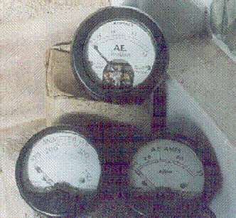
A similar argument can be applied to any oscillation, even if it is not sinusoidal, but the determination of the rms value of a waveform which is not sinusoidal from the shape of the waveform requires a knowledge of its frequency components. Happily, it is possible to measure the rms value of the current produced by such a wave directly, as the rms value is equal to the direct current (dc) e.g. from a battery which will produce an equal heating effect. Instruments such as Duddell's thermo-galvanometer convert current into heat and use the heating effect to generate a dc output from a thermocouple (in a slightly modified form, these instruments as used today are referred to as thermocouple ammeters; three are shown here) which can be measured with a meter, and these instruments can, with some care, be used to determine the rms amplitude of any current, of any waveform, at any frequency. This even applies to waveforms which are of composite frequency and of very short duration, provided that they are repeated sufficiently often that their time average is non-zero on the timescale of the galvanometer response.
 Duddell's
thermo-galvanometer is shown to the left. Q is a quartz fibre by
means of which a small mirror M is suspended. This is joined by a
glass fibre G to a silver loop L suspended between the poles N and S
of a magnet. The end of the loop terminates in a bismuth-antimony
thermocouple Bi Sb suspended above a heater. The current to be
investigated is passed through the heater, usually a fine platinum
wire for low resistances to say 40 ohms, or a platinised glass fibre
for higher resistances and lower currents. The heater is only a few
millimetres long and hence has very low inductance and capacitance.
In modern thermocouple ammeters, the heater is a piece of resistance
wire two or three centimetres long of a composition and diameter
appropriate to the current to be measured, and a thermocouple, e.g.
copper-constantan, is joined to it at approximately its midpoint. The
leads from the thermocouple are then taken to a moving coil
microammeter of conventional construction.
Duddell's
thermo-galvanometer is shown to the left. Q is a quartz fibre by
means of which a small mirror M is suspended. This is joined by a
glass fibre G to a silver loop L suspended between the poles N and S
of a magnet. The end of the loop terminates in a bismuth-antimony
thermocouple Bi Sb suspended above a heater. The current to be
investigated is passed through the heater, usually a fine platinum
wire for low resistances to say 40 ohms, or a platinised glass fibre
for higher resistances and lower currents. The heater is only a few
millimetres long and hence has very low inductance and capacitance.
In modern thermocouple ammeters, the heater is a piece of resistance
wire two or three centimetres long of a composition and diameter
appropriate to the current to be measured, and a thermocouple, e.g.
copper-constantan, is joined to it at approximately its midpoint. The
leads from the thermocouple are then taken to a moving coil
microammeter of conventional construction.
The amplitude of a wave is hence its intensity variation with time, with or without a suitable weighting factor.
'Decrement'. Only a pure sinusoidal wave of infinite duration can be said to have one single spot frequency. As the duration is reduced, so the frequency spectrum of the wave is broadened according to the Heisenberg uncertainty principle. Normally, the difference this makes for communication purposes is relatively trivial (try telling that to a mobile phone company!) but in some applications, e.g. radar and Fourier transform nuclear magnetic resonance spectroscopy (the MRI scanners used in hospitals are an example with which many people will be familiar) which both employ pulses of very short duration, the effect is of great importance. It was also of vital significance during the years of spark.
The emissions from the LC tuned circuits of a spark transmitter have the characteristic of short bursts of oscillation separated by gaps of inactivity. Each of these bursts, called "jigs" by Marconi, consists of a sinusoidal oscillation, the peak amplitude of which decreases with time according to an exponential law, the precise constants of which are determined by the resistive losses in the tuned circuit generating the oscillations and in the "radiation resistance" of the aerial through which these bursts of energy are "lost" as electromagnetic radiation. Decrement, often called logarithmic decrement, is a measure of how rapidly the peak amplitude of the wave decays, of how rapidly the oscillating circuit and/or aerial loses its energy, and hence how broad the frequency spectrum will be, and it is from this vital fact - that measuring the decrement (which is easy to do) gives a figure of merit for the broadness or narrowness of the frequency distribution (which in the early days was very difficult to observe) that the decrement of a wave became a useful quantity to know. Logarithmic decrement was the Victorian spectrum analyser. It is thus related to another two useful quantities, the loaded "Q" of the system and the "damping" as described later. From around 1910, laws were passed in all active transmitting nations limiting the decrement of the waves emitted by transmitters, and the commonly accepted upper limit was 0.2, being equivalent to 23 (or 24, depending on how you calculated it) complete oscillations from the start of the burst of oscillation to the point at which the peak amplitude was reduced to 1% of the initial peak amplitude.
The above graphs give a good idea of firstly a barely legal emission with the maximum permitted decrement of 0.2, a decidedly illegal emission with a decrement of 0.53 and an emission having a value of decrement which good operators were able to achieve in practice, 0.09. In fact, these examples have been chosen with a purpose as we shall see later. The value of logarithmic decrement, though great, was not without its shortcomings. A persistent wave of high harmonic content, e.g. a sawtooth or square wave, could have a low decrement, but be capable of causing severe interference, and this of course was the case with arc transmitters, which, though they produced continuous oscillations which did not die away in short bursts, nevertheless managed to generate not one sinusoidal oscillation, but a vast number at different frequencies all at once. Decrement therefore was a term which originated with spark transmissions and had its greatest significance in relation to the logarithmically-decaying sinusoidal oscillations associated with the intermittent charge/discharge cycles of the resonant circuits in them.
There is a simple relationship between decrement and the value of loaded Q in a tuned circuit:
![]()
from which it can be seen that d, the logarithmic decrement, is a measure of the energy lost in circuit resistance (or consumed by coupling into a load which has an effective resistance) in proportion to the energy stored in the circuit. This is also equal to
![]()
where the currents I1, I3, I5 and I7 (etc) are the currents of successive maxima (the even numbered currents correspond to the minima and could in fact be substituted just as well) and d is the logarithmic decrement, defined as the natural logarithm (log to base e, written ln) of the ratio of successive maxima. This can be expressed in exponential terms of the ratio of successive maxima (or minima) in an exponentially-decaying wavetrain:
![]()
The number of oscillations m in a wavetrain to the 1% of initial amplitude limit is given by the equation:
![]()
If the number of oscillations is large, d is small, and this simplifies to:
![]()
and hence two different answers may be obtained for the number of complete cycles in a wavetrain. This same thinking can be used to obtain Q if a decaying wavetrain can be recorded in some way. Let the number of complete cycles to the point of 50% decay equal m50. Then:
![]()
Since one complete cycle contains one maximum and one minimum, the problem of determining complete cycles is reduced to one of counting the number of maxima (or minima).
'Damping.' The equation which describes the damped oscillations shown in the above graphs is:
![]()
Here, E is the initial voltage, L the inductance, w (omega) equal to 2pf and t the time. The factora is called the damping of the circuit and is given by:
![]()
where R is the resistance in the circuit. Note that it is not possible to decide by looking at the value of decrement d, loaded Q or dampinga whether the resistance R brings about a thermal loss of energy and thus is the cause of inefficiency (i2R losses in the coils, connections, spark gap and to a lesser extent the capacitors) or is the reflected resistance into the circuit of e.g. an aerial (or Tesla coil) by which energy is lost as radiation (or sparks), which adds to the efficiency of the station in communicating. As far as these quantities are concerned, R is simply the means by which energy "escapes" from the system.
'Find the resonant frequency of a circuit consisting of a coil of 500 microhenries inductance in series with a capacitor of 2,000 picofarads.'
If the resistance in a tuned circuit is negligible, then the resonant frequency is given by the well-known formula:
![]()
where L is the circuit inductance and C the circuit capacitance. Therefore the resonant frequency of 500mH plus 2000pF is 159kc/s (post-moderns may prefer this in kHz: I am not a post-modern, the numbers are identical in both cases and anyway this is a 1954 exam paper, so kilocycles per second it is!)
This concludes the basics of the spark transmitter, but as we shall see there is still a long way to go. I have also failed miserably to answer the question in twenty minutes, thus falling short of even Second Class Wireless Operator standards: however, I plead belligerent modern technology in the form of formula editor, spreadsheet and graph creation software, and an utterly fascist html creator which insists on automatically modifying things I type without either asking me or allowing me to turn it off (thanks Star Office).
In the next section we shall look at how to build a quenched spark gap.